Chapter 5 Worked normalization examples

We will demonstrate exploratory normalization steps on the expression datasets.

5.1 Setup: download supplementary files

5.2 load Some data

library(GEOquery)

## Loading required package: Biobase

## Loading required package: BiocGenerics

## Loading required package: generics

## 
## Attaching package: 'generics'

## The following objects are masked from 'package:base':
## 
##     as.difftime, as.factor, as.ordered, intersect, is.element, setdiff,
##     setequal, union

## 
## Attaching package: 'BiocGenerics'

## The following objects are masked from 'package:stats':
## 
##     IQR, mad, sd, var, xtabs

## The following objects are masked from 'package:base':
## 
##     anyDuplicated, aperm, append, as.data.frame, basename, cbind,
##     colnames, dirname, do.call, duplicated, eval, evalq, Filter, Find,
##     get, grep, grepl, is.unsorted, lapply, Map, mapply, match, mget,
##     order, paste, pmax, pmax.int, pmin, pmin.int, Position, rank,
##     rbind, Reduce, rownames, sapply, saveRDS, table, tapply, unique,
##     unsplit, which.max, which.min

## Welcome to Bioconductor
## 
##     Vignettes contain introductory material; view with
##     'browseVignettes()'. To cite Bioconductor, see
##     'citation("Biobase")', and for packages 'citation("pkgname")'.

## Setting options('download.file.method.GEOquery'='auto')

## Setting options('GEOquery.inmemory.gpl'=FALSE)

library(knitr)
library(dplyr)

## 
## Attaching package: 'dplyr'

## The following object is masked from 'package:Biobase':
## 
##     combine

## The following objects are masked from 'package:BiocGenerics':
## 
##     combine, intersect, setdiff, setequal, union

## The following object is masked from 'package:generics':
## 
##     explain

## The following objects are masked from 'package:stats':
## 
##     filter, lag

## The following objects are masked from 'package:base':
## 
##     intersect, setdiff, setequal, union

library(tibble)
if(!require(tidyverse)){
  install.packages("tidyvers",dependencies = FALSE)
}

## Loading required package: tidyverse

## Error: package or namespace load failed for 'tidyverse':
##  .onAttach failed in attachNamespace() for 'tidyverse', details:
##   call: library(pkg, lib.loc = loc, character.only = TRUE, warn.conflicts = FALSE)
##   error: there is no package called 'lubridate'

## Installing package into '/usr/local/lib/R/site-library'
## (as 'lib' is unspecified)

## Warning: package 'tidyvers' is not available for this version of R
## 
## A version of this package for your version of R might be available elsewhere,
## see the ideas at
## https://cran.r-project.org/doc/manuals/r-patched/R-admin.html#Installing-packages

library(tidyverse)

gse <- "GSE119732"

source("./supp_functions.R")
fetch_geo_supp(gse = gse)

## Using locally cached version of supplementary file(s) GSE119732 found here:
## data/GSE119732/GSE119732_count_table_RNA_seq.txt.gz

path <- file.path("data", gse)
files <- list.files(path, pattern = "\\.txt.gz$|\\.tsv.gz$|\\.csv.gz$", 
                    full.names = TRUE, recursive = TRUE)

Raw table preview

library(readr)

safe_read <- function(file) {
  # First attempt: read as TSV
  df <- tryCatch(
    readr::read_tsv(file, show_col_types = FALSE),
    error = function(e) NULL   # catch fatal errors
  )
  
  # If read_tsv failed entirely:
  if (is.null(df)) {
    message("TSV read failed — reading as space-delimited file instead.")
    return(readr::read_table(file, show_col_types = FALSE))
  }
  
  # If read_tsv returned but with parsing issues:
  probs <- problems(df)
  if (nrow(probs) > 0) {
    message("Parsing issues detected in TSV — reading as space-delimited file instead.")
    return(readr::read_table(file, show_col_types = FALSE))
  }
  
  # If everything was fine:
  return(df)
}

x <- safe_read(files[1])


kable_head(x[, 1:min(6, ncol(x))], 5, paste(gse,": raw table preview"))

(#tab:preview_raw)GSE119732 : raw table preview

gene_id	A1	A2	A3	A4	B1
ENSG00000223972.5	0	0	0	0	0
ENSG00000227232.5	79	119	84	50	80
ENSG00000278267.1	17	10	22	19	19
ENSG00000243485.4	0	0	0	0	0
ENSG00000237613.2	0	0	0	0	0

5.3 Example 1: GSE119732

Before doing anything to this data. What does it look like?

plot_box(x[,2:ncol(x)])

plot_density(x[,2:ncol(x)])

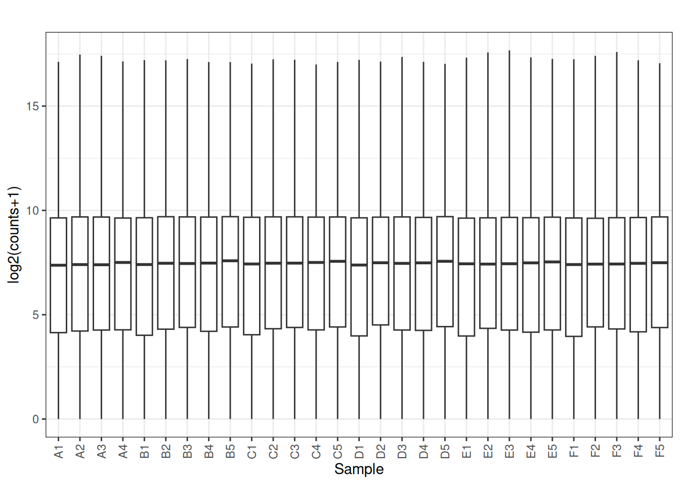
5.4 Convert the raw counts to Counts per million (CPM)

library(edgeR)

## Loading required package: limma

## 
## Attaching package: 'limma'

## The following object is masked from 'package:BiocGenerics':
## 
##     plotMA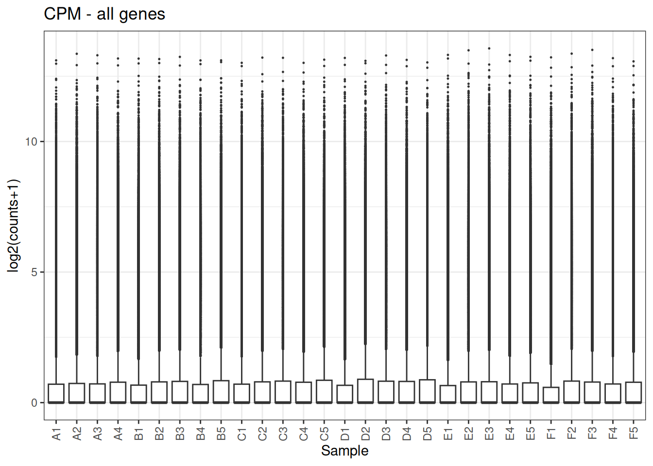

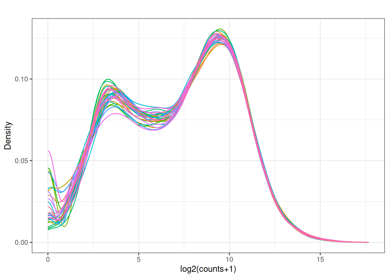
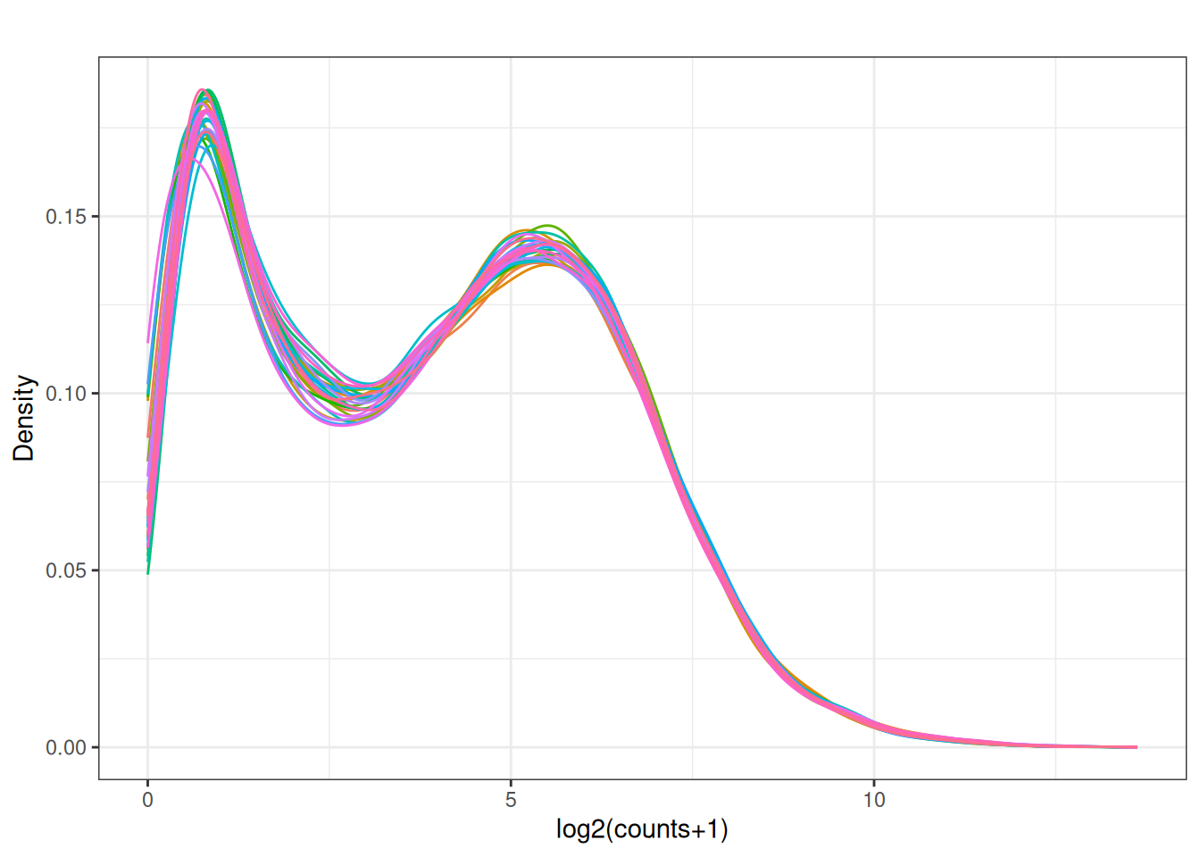
x_cpm <- cpm(y = x[,2:ncol(x)])

plot_box(x_cpm,main = "CPM - all genes")

Visualize as a density plot as well

plot_density(x_cpm,main = "CPM - all genes, NO design")

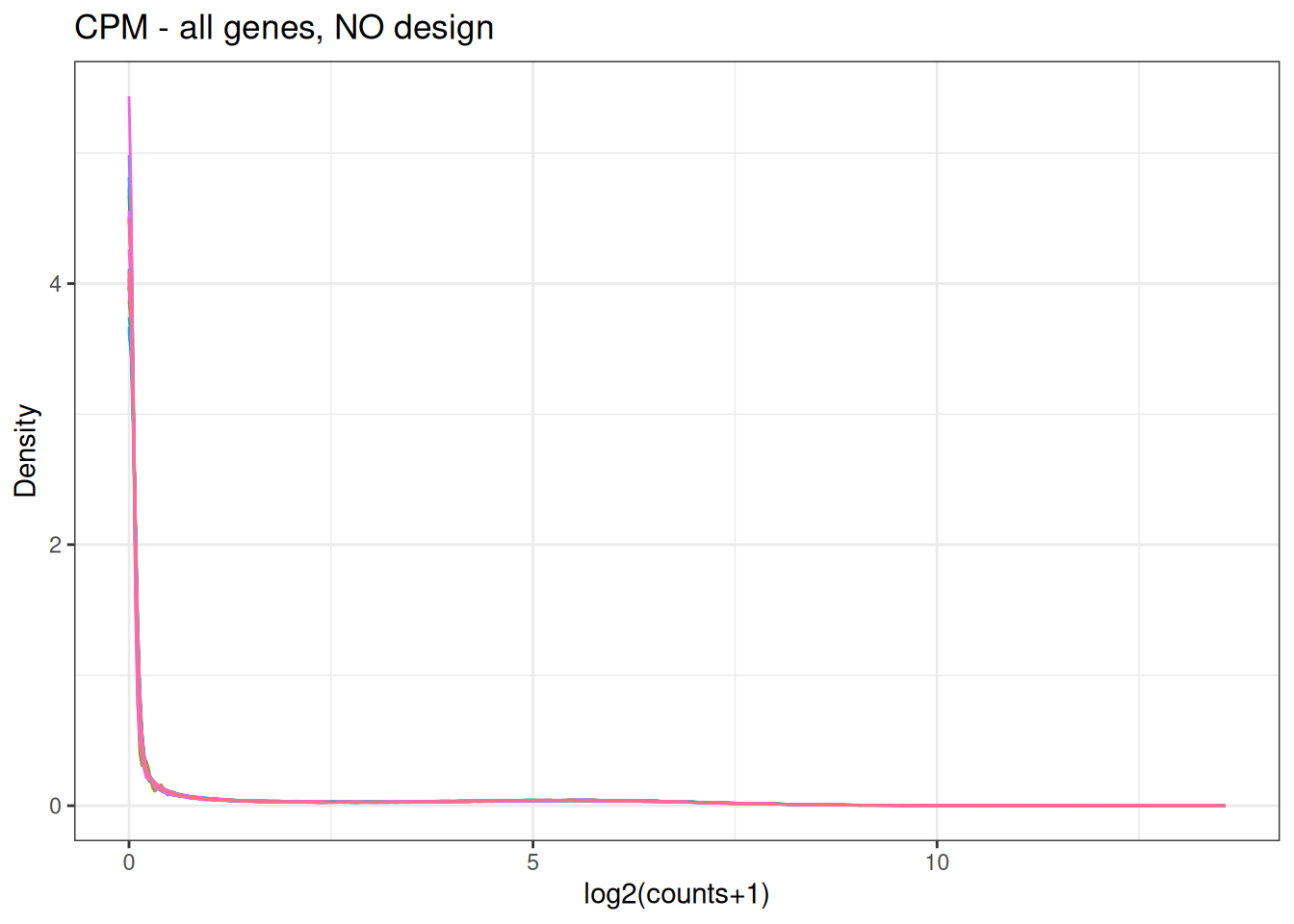
There are a lot of genes that have zero expression. That is the majority of them. So we need to get rid of them.

5.5 filter out lowly expressed genes

to_remove <- edgeR::filterByExpr(x_cpm,min.count = 3)

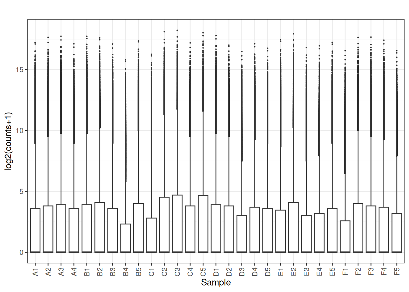
## No group or design set. Assuming all samples belong to one group.

x_cpm_filtered <- x_cpm[to_remove,]

plot_box(x_cpm_filtered,main = "CPM filtered out lowly expressed - \nNO design matrix")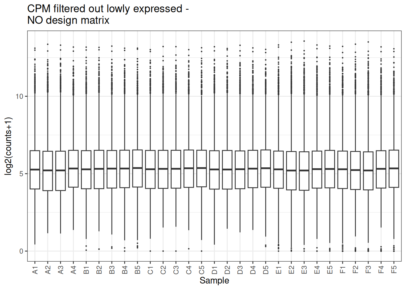

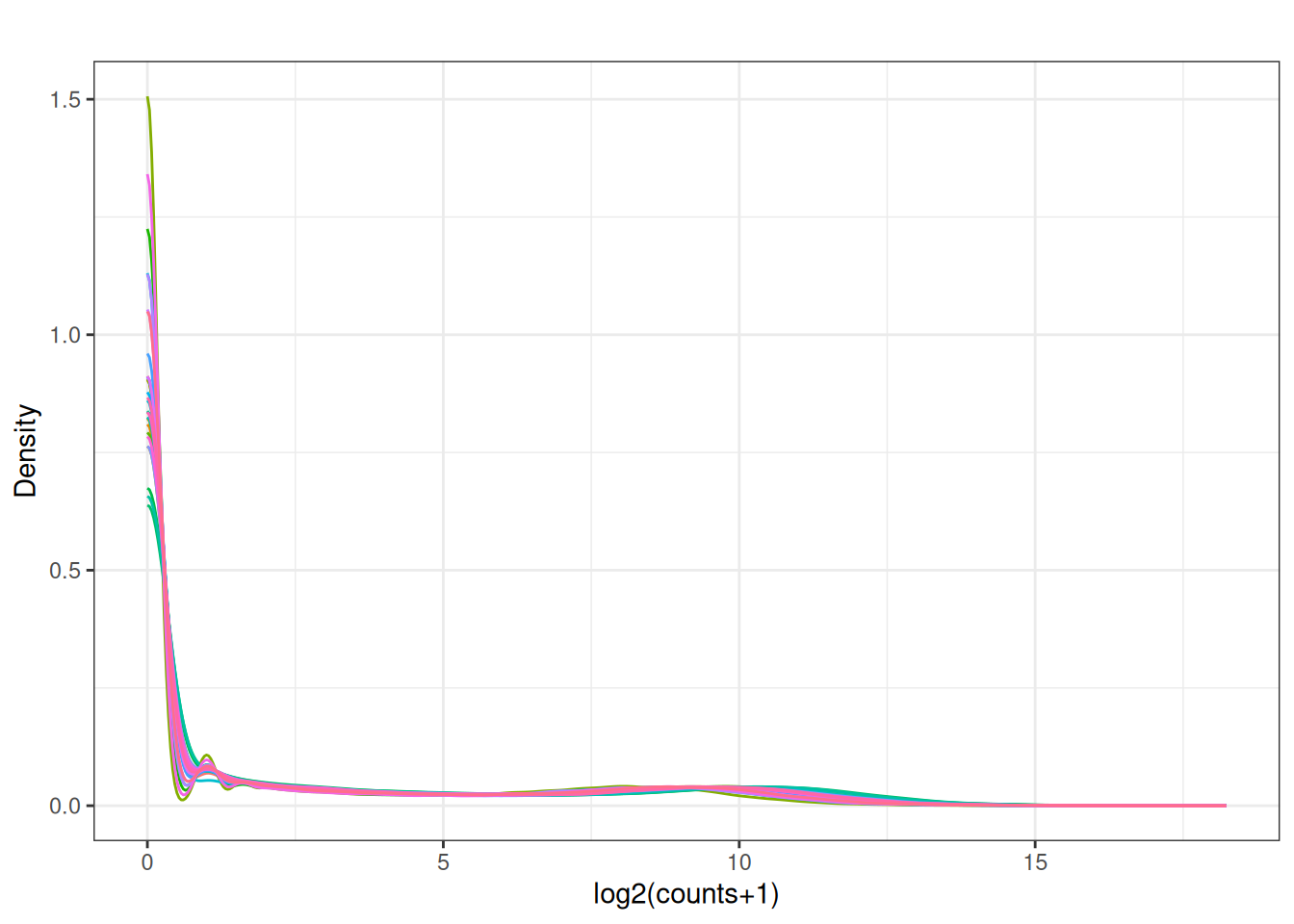
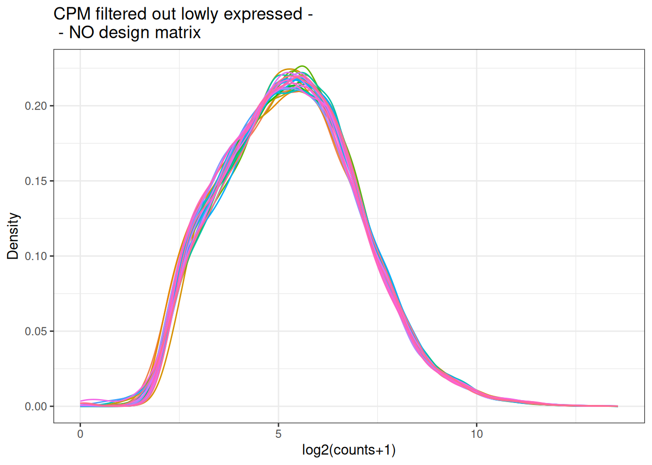
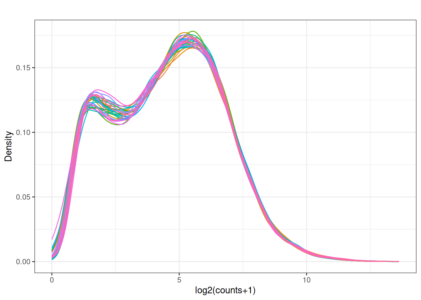
visualize this as density plot as well.

plot_density(x_cpm_filtered,main = "CPM filtered out lowly expressed - \n - NO design matrix")

5.6 Incorporate a design matrix - description of the samples.

The above was usingn all of the samples the same but this dataset has varying sample types. I might be hard to figure it out just from column names as they are not so informative but let’s just guess

colnames(x)

##  [1] "gene_id" "A1"      "A2"      "A3"      "A4"      "B1"      "B2"     
##  [8] "B3"      "B4"      "B5"      "C1"      "C2"      "C3"      "C4"     
## [15] "C5"      "D1"      "D2"      "D3"      "D4"      "D5"      "E1"     
## [22] "E2"      "E3"      "E4"      "E5"      "F1"      "F2"      "F3"     
## [29] "F4"      "F5"

#design matrix - 
samples <- colnames(x)[2:ncol(x)]
patient  <- substr(samples, 1, 1)       
celltype <- substr(samples, 2, nchar(samples))   
sample_data <- data.frame(samples, patient, celltype)


design <- model.matrix(~ 0 + celltype,data = sample_data)
rownames(design) <- sample_data$samples
colnames(design) <- paste0("celltype", levels(factor(celltype)))
design

##    celltype1 celltype2 celltype3 celltype4 celltype5
## A1         1         0         0         0         0
## A2         0         1         0         0         0
## A3         0         0         1         0         0
## A4         0         0         0         1         0
## B1         1         0         0         0         0
## B2         0         1         0         0         0
## B3         0         0         1         0         0
## B4         0         0         0         1         0
## B5         0         0         0         0         1
## C1         1         0         0         0         0
## C2         0         1         0         0         0
## C3         0         0         1         0         0
## C4         0         0         0         1         0
## C5         0         0         0         0         1
## D1         1         0         0         0         0
## D2         0         1         0         0         0
## D3         0         0         1         0         0
## D4         0         0         0         1         0
## D5         0         0         0         0         1
## E1         1         0         0         0         0
## E2         0         1         0         0         0
## E3         0         0         1         0         0
## E4         0         0         0         1         0
## E5         0         0         0         0         1
## F1         1         0         0         0         0
## F2         0         1         0         0         0
## F3         0         0         1         0         0
## F4         0         0         0         1         0
## F5         0         0         0         0         1
## attr(,"assign")
## [1] 1 1 1 1 1
## attr(,"contrasts")
## attr(,"contrasts")$celltype
## [1] "contr.treatment"

Filter use design information

to_remove_withdesign <- edgeR::filterByExpr(x_cpm,min.count = 3,
                                            design = design)
x_cpm_filtered_withdesign <- x_cpm[to_remove_withdesign,]

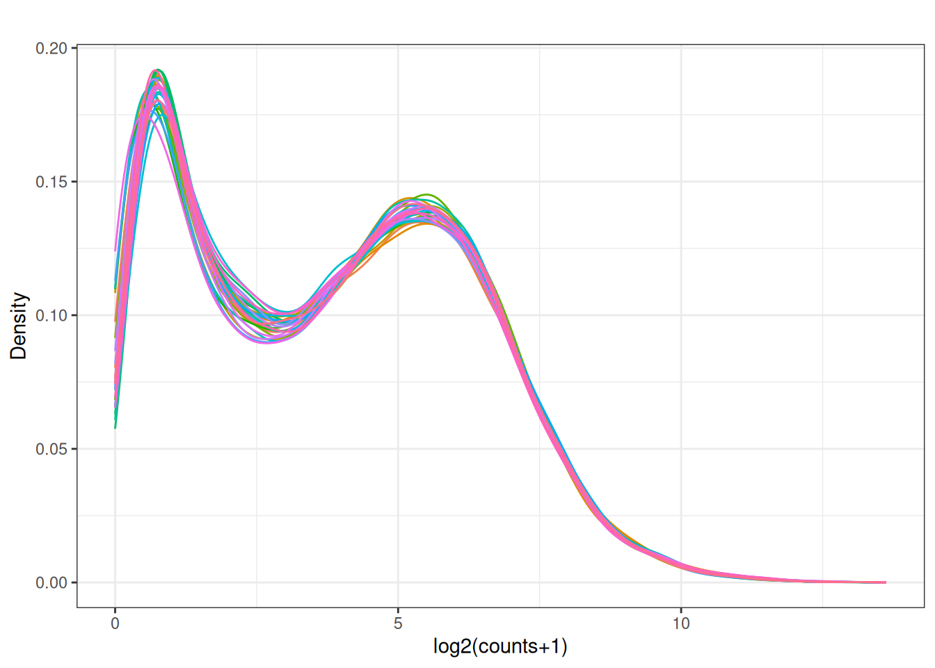
plot_box(x_cpm_filtered_withdesign,main = "CPM filtered out lowly expressed - \n - with design matrix")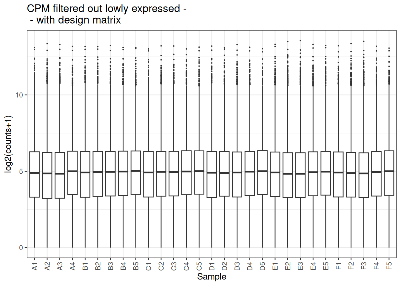

plot_density(x_cpm_filtered_withdesign,main = "CPM filtered out lowly expressed - \n - with design matrix")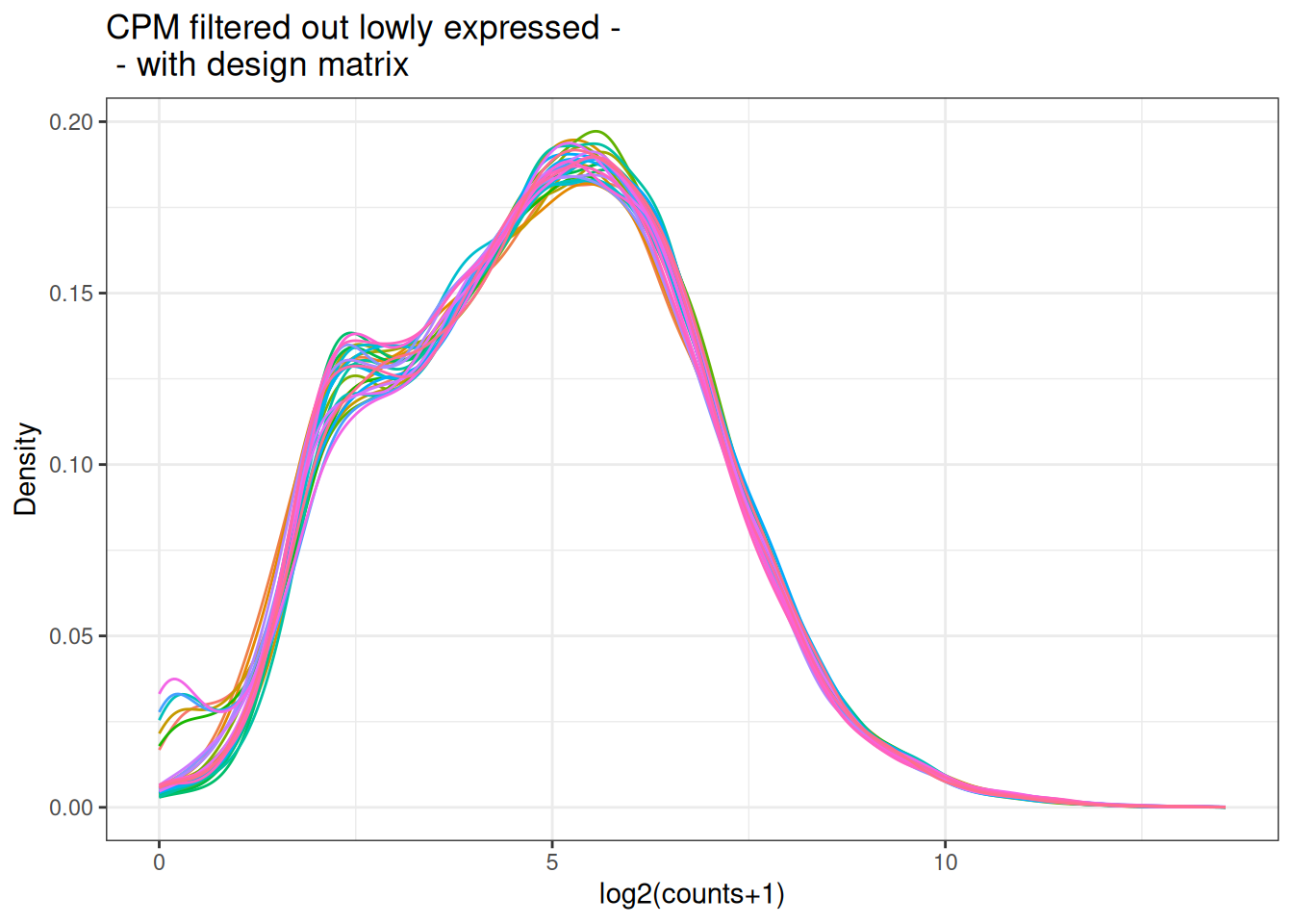

5.7 Normalize Dataset using TMM

library(edgeR)

dge <- DGEList(counts = x[,2:ncol(x)])
dge_filtered <- dge[filterByExpr(dge),]

## Warning in filterByExpr.DGEList(dge): All samples appear to belong to the same
## group.

dge_filtered  <- calcNormFactors(dge_filtered , method = "TMM")
norm_cpm <- cpm(dge_filtered , log = FALSE, prior.count = 1)

plot_box(norm_cpm)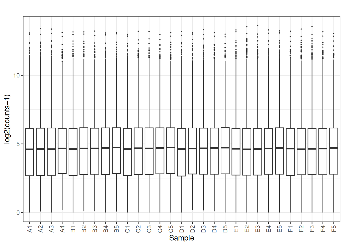

plot_density(norm_cpm)

5.8 Look at the distribution of our samples in 2D space

y <- dge_filtered

plotMDS(y, top = 500, labels = colnames(y), 
       col = as.integer(y$samples$group))
legend("topright", legend = levels(y$samples$group),
       col = seq_along(levels(y$samples$group)), pch = 16, bty = "n")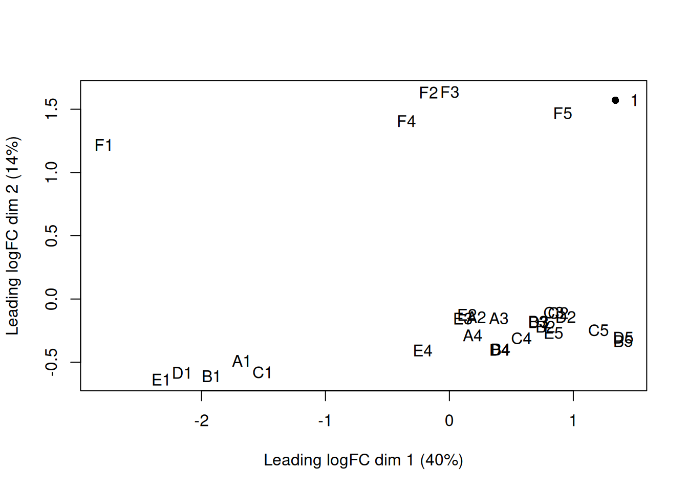

Now incorporate the design into the process

dge <- DGEList(counts = x[,2:ncol(x)],group = sample_data$celltype)
dge_filtered <- dge[filterByExpr(dge),]
dge_filtered  <- calcNormFactors(dge_filtered , method = "TMM")
norm_cpm <- cpm(dge_filtered , log = FALSE, prior.count = 1)

plot_box(norm_cpm)

plot_density(norm_cpm)

y <- dge_filtered

plotMDS(y, top = 500, labels = colnames(y), 
       col = as.integer(y$samples$group))
legend("topright", legend = levels(y$samples$group),
       col = seq_along(levels(y$samples$group)), pch = 16, bty = "n")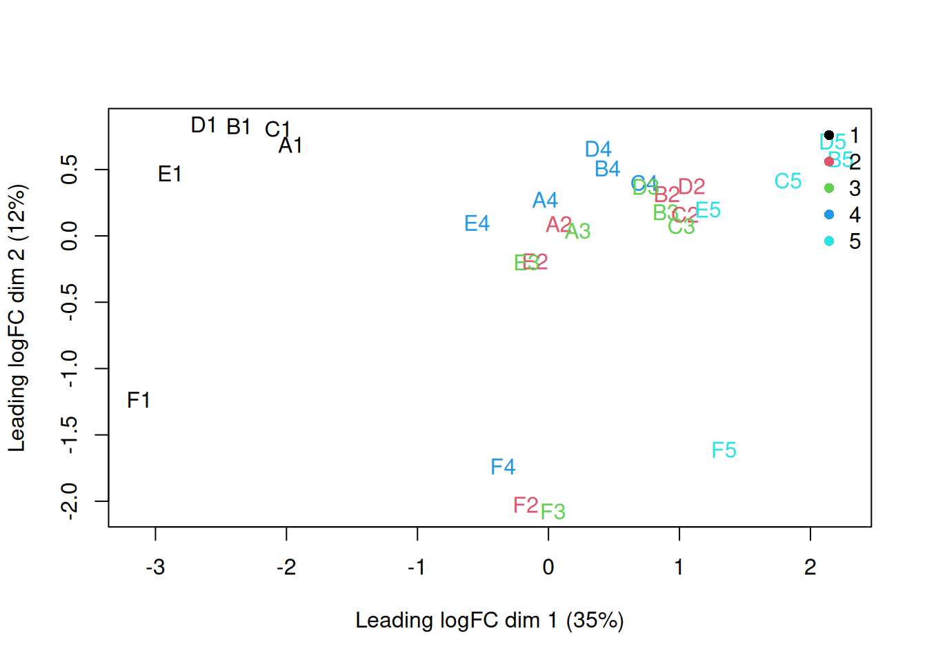

Now incorporate the design into the process

dge <- DGEList(counts = x[,2:ncol(x)],group = sample_data$patient)
dge_filtered <- dge[filterByExpr(dge),]
dge_filtered  <- calcNormFactors(dge_filtered , method = "TMM")
norm_cpm <- cpm(dge_filtered , log = FALSE, prior.count = 1)

plot_box(norm_cpm)

plot_density(norm_cpm)

y <- dge_filtered

plotMDS(y, top = 500, labels = colnames(y), 
       col = as.integer(y$samples$group))
legend("topright", legend = levels(y$samples$group),
       col = seq_along(levels(y$samples$group)), pch = 16, bty = "n")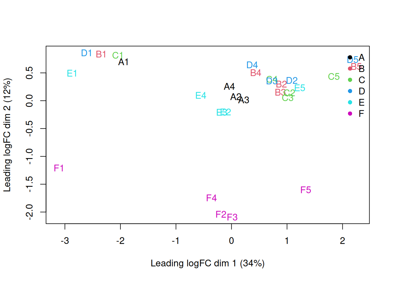

5.9 Normalize the Dataset using RLE

library(DESeq2)

## Loading required package: S4Vectors

## Loading required package: stats4

## 
## Attaching package: 'S4Vectors'

## The following object is masked from 'package:tidyr':
## 
##     expand

## The following objects are masked from 'package:dplyr':
## 
##     first, rename

## The following object is masked from 'package:utils':
## 
##     findMatches

## The following objects are masked from 'package:base':
## 
##     expand.grid, I, unname

## Loading required package: IRanges

## 
## Attaching package: 'IRanges'

## The following object is masked from 'package:purrr':
## 
##     reduce

## The following objects are masked from 'package:dplyr':
## 
##     collapse, desc, slice

## Loading required package: GenomicRanges

## Loading required package: GenomeInfoDb

## Loading required package: SummarizedExperiment

## Loading required package: MatrixGenerics

## Loading required package: matrixStats

## 
## Attaching package: 'matrixStats'

## The following object is masked from 'package:dplyr':
## 
##     count

## The following objects are masked from 'package:Biobase':
## 
##     anyMissing, rowMedians

## 
## Attaching package: 'MatrixGenerics'

## The following objects are masked from 'package:matrixStats':
## 
##     colAlls, colAnyNAs, colAnys, colAvgsPerRowSet, colCollapse,
##     colCounts, colCummaxs, colCummins, colCumprods, colCumsums,
##     colDiffs, colIQRDiffs, colIQRs, colLogSumExps, colMadDiffs,
##     colMads, colMaxs, colMeans2, colMedians, colMins, colOrderStats,
##     colProds, colQuantiles, colRanges, colRanks, colSdDiffs, colSds,
##     colSums2, colTabulates, colVarDiffs, colVars, colWeightedMads,
##     colWeightedMeans, colWeightedMedians, colWeightedSds,
##     colWeightedVars, rowAlls, rowAnyNAs, rowAnys, rowAvgsPerColSet,
##     rowCollapse, rowCounts, rowCummaxs, rowCummins, rowCumprods,
##     rowCumsums, rowDiffs, rowIQRDiffs, rowIQRs, rowLogSumExps,
##     rowMadDiffs, rowMads, rowMaxs, rowMeans2, rowMedians, rowMins,
##     rowOrderStats, rowProds, rowQuantiles, rowRanges, rowRanks,
##     rowSdDiffs, rowSds, rowSums2, rowTabulates, rowVarDiffs, rowVars,
##     rowWeightedMads, rowWeightedMeans, rowWeightedMedians,
##     rowWeightedSds, rowWeightedVars

## The following object is masked from 'package:Biobase':
## 
##     rowMedians

counts <- x[,2:ncol(x)]

keep <- rowSums(counts >= 10) >= 2
counts_filtered <- counts[keep, ]

dds <- DESeqDataSetFromMatrix(countData = counts_filtered, 
                              colData = sample_data,
                              design = design)

## converting counts to integer mode

dds <- estimateSizeFactors(dds)

norm_counts <- counts(dds, normalized = TRUE)

plot_box(norm_counts)

plot_density(norm_counts)