Chapter 9 Differential expression with limma-voom - Dataset 2
In this chapter we run limma-voom, which:
- Starts from raw counts
- Transforms to log2-CPM with precision weights (
voom()) - Fits a linear model + empirical Bayes moderation
We use an additive model:
\[ \text{expression} \sim \text{cellline} + \text{treatment} \]
This estimates treatment effects while controlling for baseline differences between cell lines.
obj <- readRDS("data/d2_qc_objects.rds")
dge_f <- obj$dge_f
meta <- obj$meta
mappings <- obj$mappings

design <- obj$design

v <- limma::voom(dge_f, design, plot = TRUE)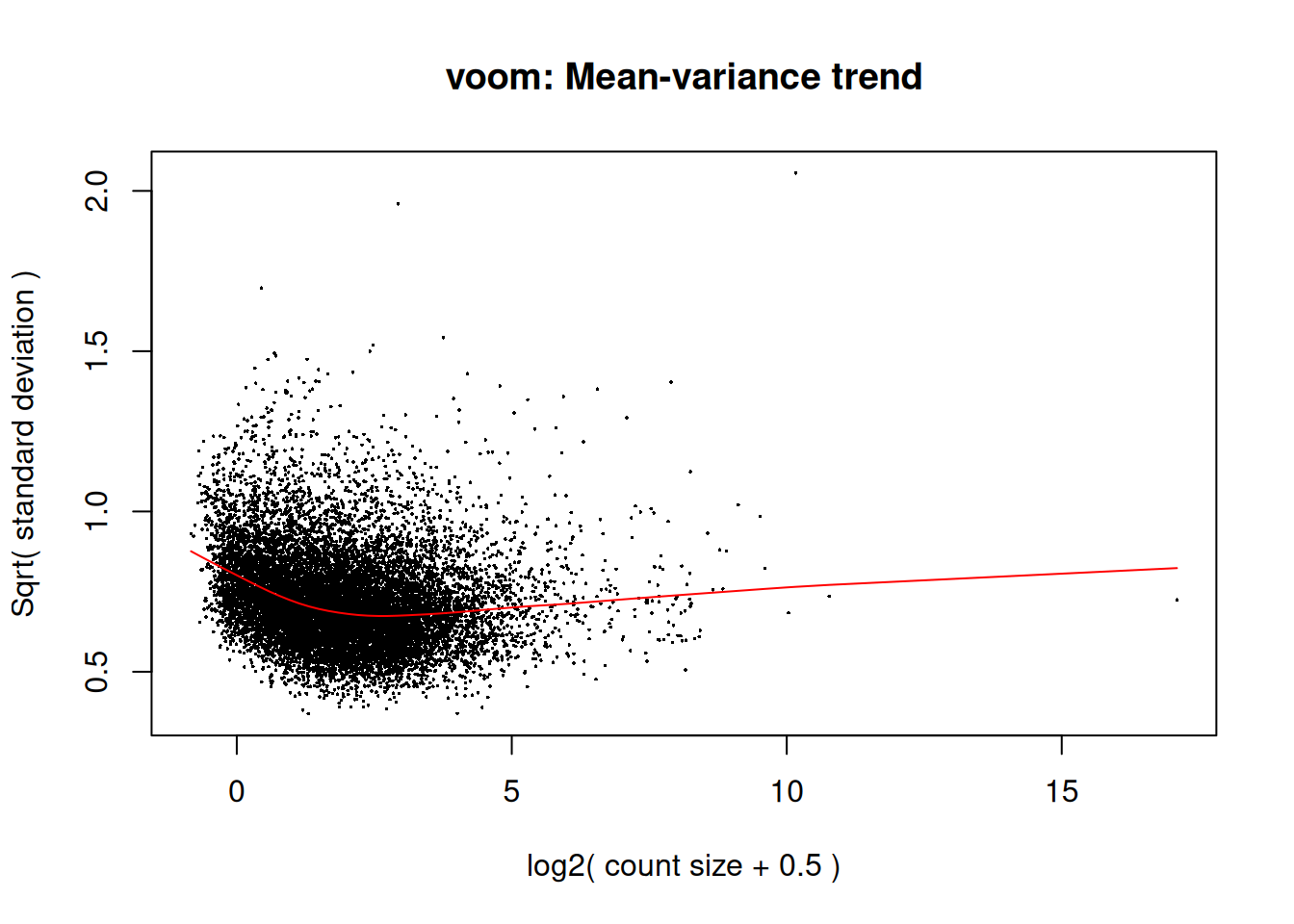
fit <- limma::lmFit(v, design)
fit <- limma::eBayes(fit, trend = TRUE)

# Contrasts
contr <- limma::makeContrasts(
  `status0` = status0 - (status1),
  levels = design
)

fit2 <- limma::contrasts.fit(fit, contr)
fit2 <- limma::eBayes(fit2, trend = TRUE)
9.1 Results tables
res_0_vs_1 <- limma::topTable(fit2, coef = "status0", number = Inf, sort.by = "P")

head(res_0_vs_1 )
## logFC AveExpr t P.Value adj.P.Val B
## ENSG00000151729.10 0.7716211 3.208481 4.456881 0.0003039356 0.9668082 -3.490636
## ENSG00000213316.9 1.0587958 2.072318 4.216054 0.0005182912 0.9668082 -3.685744
## ENSG00000138829.11 -1.3959423 2.556387 -4.213800 0.0005208933 0.9668082 -3.633678
## ENSG00000113328.18 0.6185947 6.437853 4.105158 0.0006632631 0.9668082 -3.705772
## ENSG00000211956.2 2.0603342 2.117546 4.102268 0.0006675426 0.9668082 -3.659265
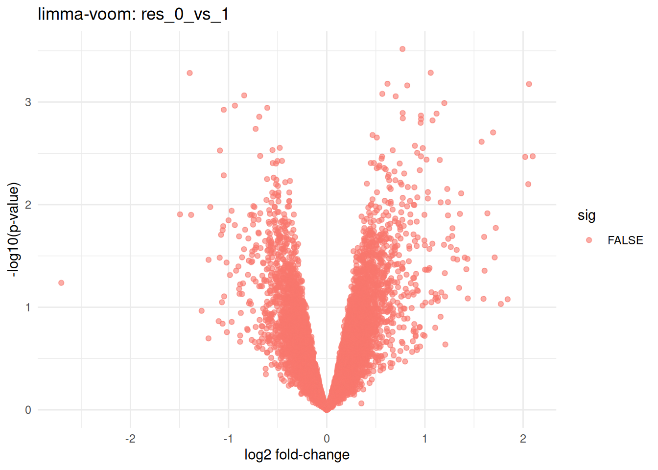
## ENSG00000152092.15 0.8195556 1.580981 4.088099 0.0006889341 0.9668082 -3.7039619.2 Volcano plot (0 vs rest)
volcano_df <- res_0_vs_1  %>%
  rownames_to_column("ensembl") %>%
  mutate(sig = adj.P.Val < 0.05)

ggplot(volcano_df, aes(x = logFC, y = -log10(P.Value), color = sig)) +
  geom_point(alpha = 0.6) +
  theme_minimal() +
  labs(
    title = "limma-voom: res_0_vs_1 ",
    x = "log2 fold-change",
    y = "-log10(p-value)"
  )