Chapter 3 Visualizing distributions

Before choosing a normalization method, inspect data distributions.

3.1 load Some data

library(GEOquery)

## Loading required package: Biobase

## Loading required package: BiocGenerics

## Loading required package: generics

## 
## Attaching package: 'generics'

## The following objects are masked from 'package:base':
## 
##     as.difftime, as.factor, as.ordered, intersect, is.element, setdiff,
##     setequal, union

## 
## Attaching package: 'BiocGenerics'

## The following objects are masked from 'package:stats':
## 
##     IQR, mad, sd, var, xtabs

## The following objects are masked from 'package:base':
## 
##     anyDuplicated, aperm, append, as.data.frame, basename, cbind,
##     colnames, dirname, do.call, duplicated, eval, evalq, Filter, Find,
##     get, grep, grepl, is.unsorted, lapply, Map, mapply, match, mget,
##     order, paste, pmax, pmax.int, pmin, pmin.int, Position, rank,
##     rbind, Reduce, rownames, sapply, saveRDS, table, tapply, unique,
##     unsplit, which.max, which.min

## Welcome to Bioconductor
## 
##     Vignettes contain introductory material; view with
##     'browseVignettes()'. To cite Bioconductor, see
##     'citation("Biobase")', and for packages 'citation("pkgname")'.

## Setting options('download.file.method.GEOquery'='auto')

## Setting options('GEOquery.inmemory.gpl'=FALSE)

library(knitr)
library(dplyr)

## 
## Attaching package: 'dplyr'

## The following object is masked from 'package:Biobase':
## 
##     combine

## The following objects are masked from 'package:BiocGenerics':
## 
##     combine, intersect, setdiff, setequal, union

## The following object is masked from 'package:generics':
## 
##     explain

## The following objects are masked from 'package:stats':
## 
##     filter, lag

## The following objects are masked from 'package:base':
## 
##     intersect, setdiff, setequal, union

library(tibble)
if(!require(tidyverse)){
  install.packages("tidyverse",dependencies = FALSE)
}

## Loading required package: tidyverse

## ── Attaching core tidyverse packages ──────────────────────── tidyverse 2.0.0 ──
## ✔ forcats   1.0.1     ✔ readr     2.1.6
## ✔ ggplot2   4.0.1     ✔ stringr   1.6.0
## ✔ lubridate 1.9.5     ✔ tidyr     1.3.2
## ✔ purrr     1.2.0     
## ── Conflicts ────────────────────────────────────────── tidyverse_conflicts() ──
## ✖ dplyr::combine()    masks Biobase::combine(), BiocGenerics::combine()
## ✖ dplyr::filter()     masks stats::filter()
## ✖ dplyr::lag()        masks stats::lag()
## ✖ ggplot2::Position() masks BiocGenerics::Position(), base::Position()
## ℹ Use the conflicted package (<http://conflicted.r-lib.org/>) to force all conflicts to become errors

library(tidyverse)

gse <- "GSE119732"

source("./supp_functions.R")
fetch_geo_supp(gse = gse)

path <- file.path("data", gse)
files <- list.files(path, pattern = "\\.txt.gz$|\\.tsv.gz$|\\.csv.gz$", 
                    full.names = TRUE, recursive = TRUE)

Raw table preview

library(readr)

safe_read <- function(file) {
  # First attempt: read as TSV
  df <- tryCatch(
    readr::read_tsv(file, show_col_types = FALSE),
    error = function(e) NULL   # catch fatal errors
  )
  
  # If read_tsv failed entirely:
  if (is.null(df)) {
    message("TSV read failed — reading as space-delimited file instead.")
    return(readr::read_table(file, show_col_types = FALSE))
  }
  
  # If read_tsv returned but with parsing issues:
  probs <- problems(df)
  if (nrow(probs) > 0) {
    message("Parsing issues detected in TSV — reading as space-delimited file instead.")
    return(readr::read_table(file, show_col_types = FALSE))
  }
  
  # If everything was fine:
  return(df)
}

x <- safe_read(files[1])


kable_head(x[, 1:min(6, ncol(x))], 5, paste(gse,": raw table preview"))

(#tab:preview_raw)GSE119732 : raw table preview

gene_id	A1	A2	A3	A4	B1
ENSG00000223972.5	0	0	0	0	0
ENSG00000227232.5	79	119	84	50	80
ENSG00000278267.1	17	10	22	19	19
ENSG00000243485.4	0	0	0	0	0
ENSG00000237613.2	0	0	0	0	0

3.2 Boxplots

library(tidyverse)

# suppose 'mat' is a gene x sample matrix (numeric)
plot_box <- function(mat, main = "", ylab = "log2(counts+1)") {
  df <- as.data.frame(mat)
  df_long <- df |>
    mutate(gene = rownames(df)) |>
    pivot_longer(-gene, names_to = "sample", values_to = "value") |>
    mutate(value = log2(value + 1))

  ggplot(df_long, aes(x = sample, y = value)) +
    geom_boxplot(outlier.size = 0.2) +
    theme_bw() +
    theme(axis.text.x = element_text(angle = 90, vjust = 0.5, hjust = 1)) +
    labs(title = main, x = "Sample", y = ylab)
}

plot_box(x[,2:ncol(x)])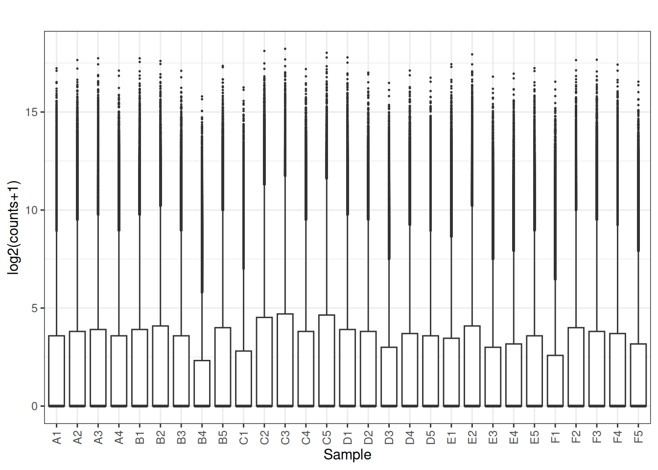

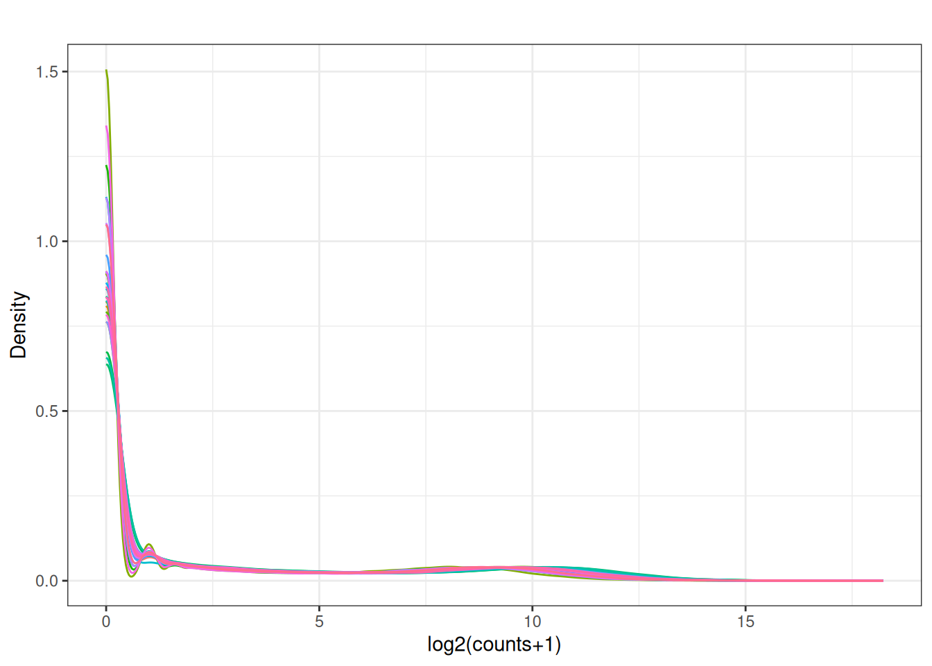
3.3 Density plots

plot_density <- function(mat, main = "") {
  df <- as.data.frame(mat)
  df_long <- df |>
    mutate(gene = rownames(df)) |>
    pivot_longer(-gene, names_to = "sample", values_to = "value") |>
    mutate(value = log2(value + 1))

  ggplot(df_long, aes(x = value, colour = sample)) +
    geom_density() +
    theme_bw() +
    labs(title = main, x = "log2(counts+1)", y = "Density") +
    guides(colour = "none")
}

plot_density(x[,2:ncol(x)])