Chapter 5 Worked normalization examples
We will demonstrate exploratory normalization steps on the expression datasets.
5.2 load Some data
Raw table preview
library(readr)

safe_read <- function(file) {
  # First attempt: read as TSV
  df <- tryCatch(
    readr::read_tsv(file, show_col_types = FALSE),
    error = function(e) NULL   # catch fatal errors
  )

  # If read_tsv failed entirely:
  if (is.null(df)) {
    message("TSV read failed — reading as space-delimited file instead.")
    return(readr::read_table(file, show_col_types = FALSE))
  }

  # If read_tsv returned but with parsing issues:
  probs <- problems(df)
  if (nrow(probs) > 0) {
    message("Parsing issues detected in TSV — reading as space-delimited file instead.")
    return(readr::read_table(file, show_col_types = FALSE))
  }

  # If everything was fine:
  return(df)
}

x <- safe_read(files[1])


kable_head(x[, 1:min(6, ncol(x))], 5, paste(gse,": raw table preview"))| Gene | T8657_900CTG_NT | T8658_1150CTG_NT | T8659_1450CTG_NT | T8660_900CTG_20CTG | T8661_1150CTG_20CTG |
|---|---|---|---|---|---|
| ENSG00000108821 | 456397 | 486088 | 608151 | 2012962 | 379186 |
| ENSG00000265150 | 170681 | 299425 | 286295 | 747000 | 210962 |
| ENSG00000164692 | 169781 | 190854 | 263391 | 869194 | 180006 |
| ENSG00000265735 | 78113 | 121697 | 113379 | 532435 | 112977 |
| ENSG00000259001 | 55081 | 78811 | 73032 | 353442 | 100823 |
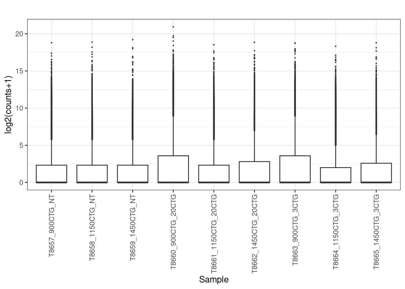
5.4 Convert the raw counts to Counts per million (CPM)
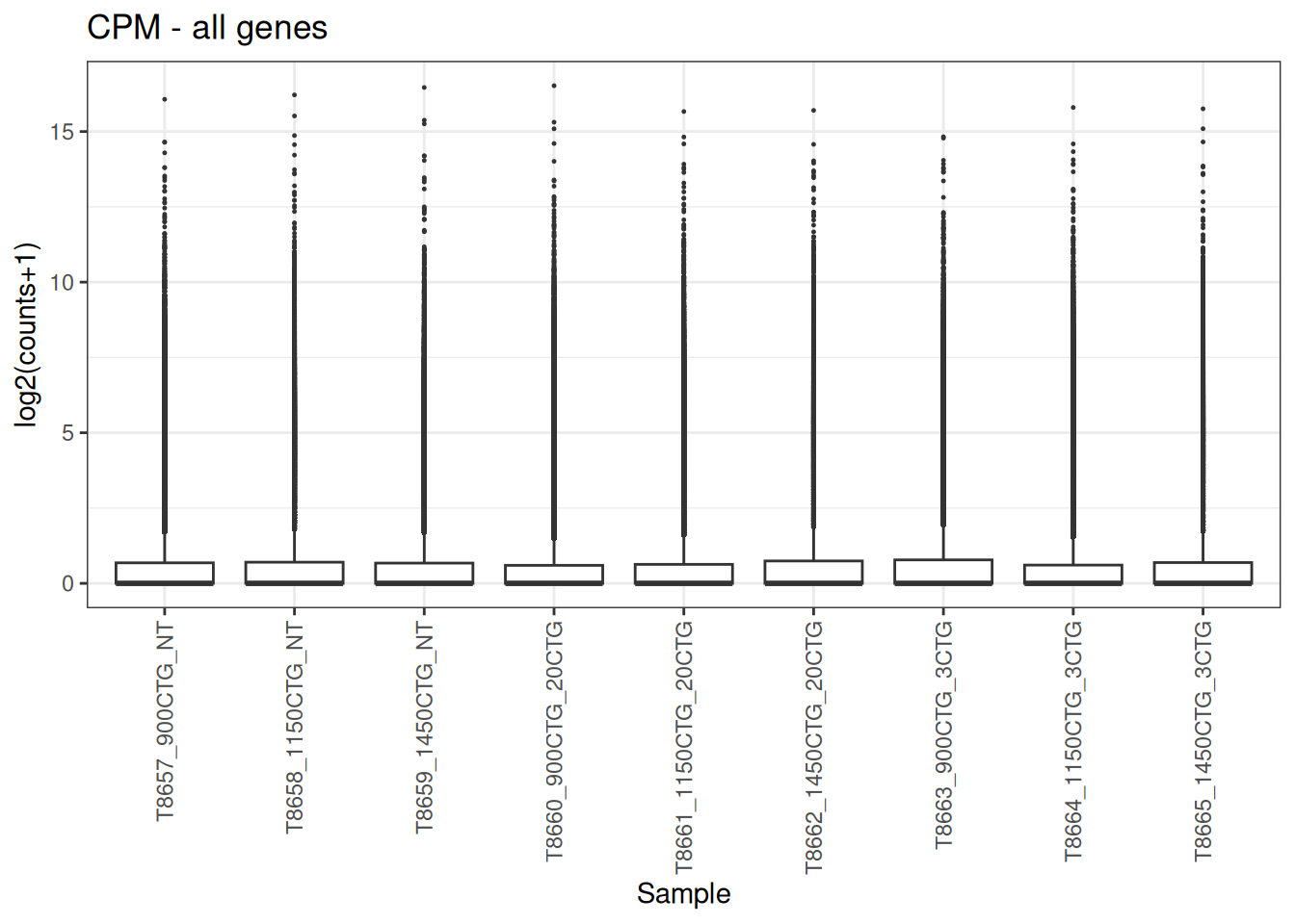
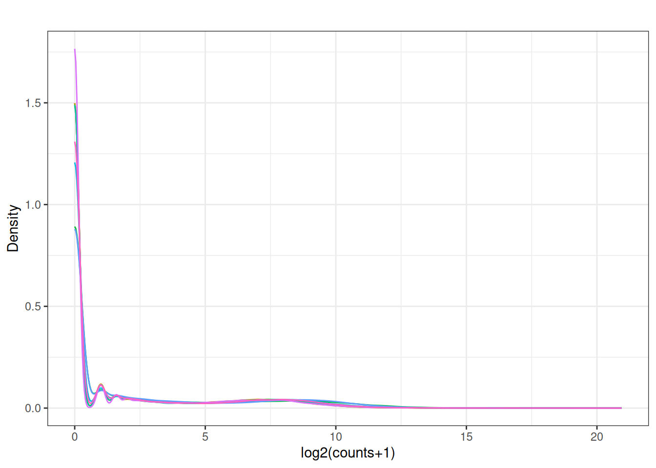
Visualize as a density plot as well
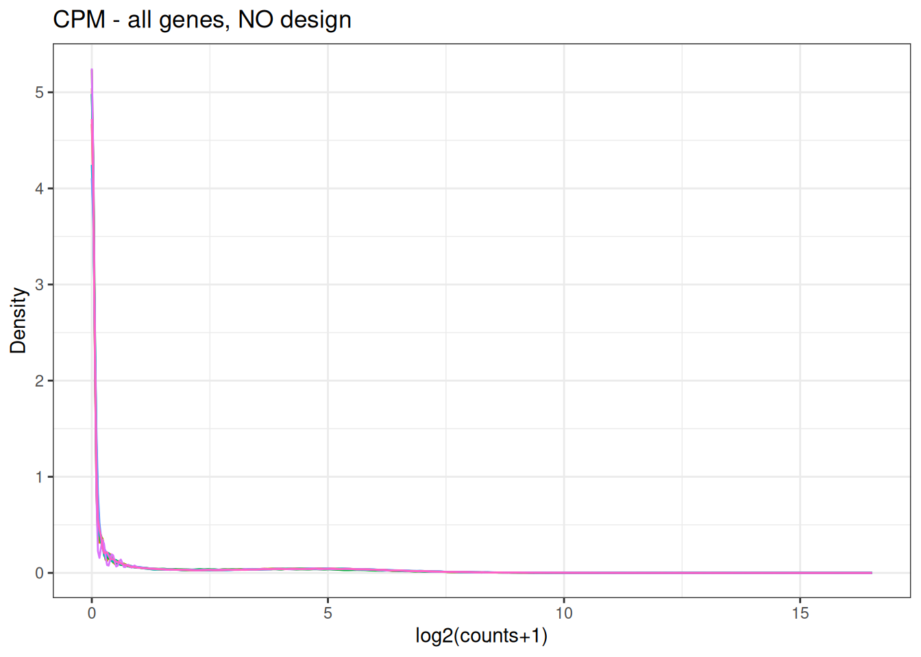
There are a lot of genes that have zero expression. That is the majority of them. So we need to get rid of them.
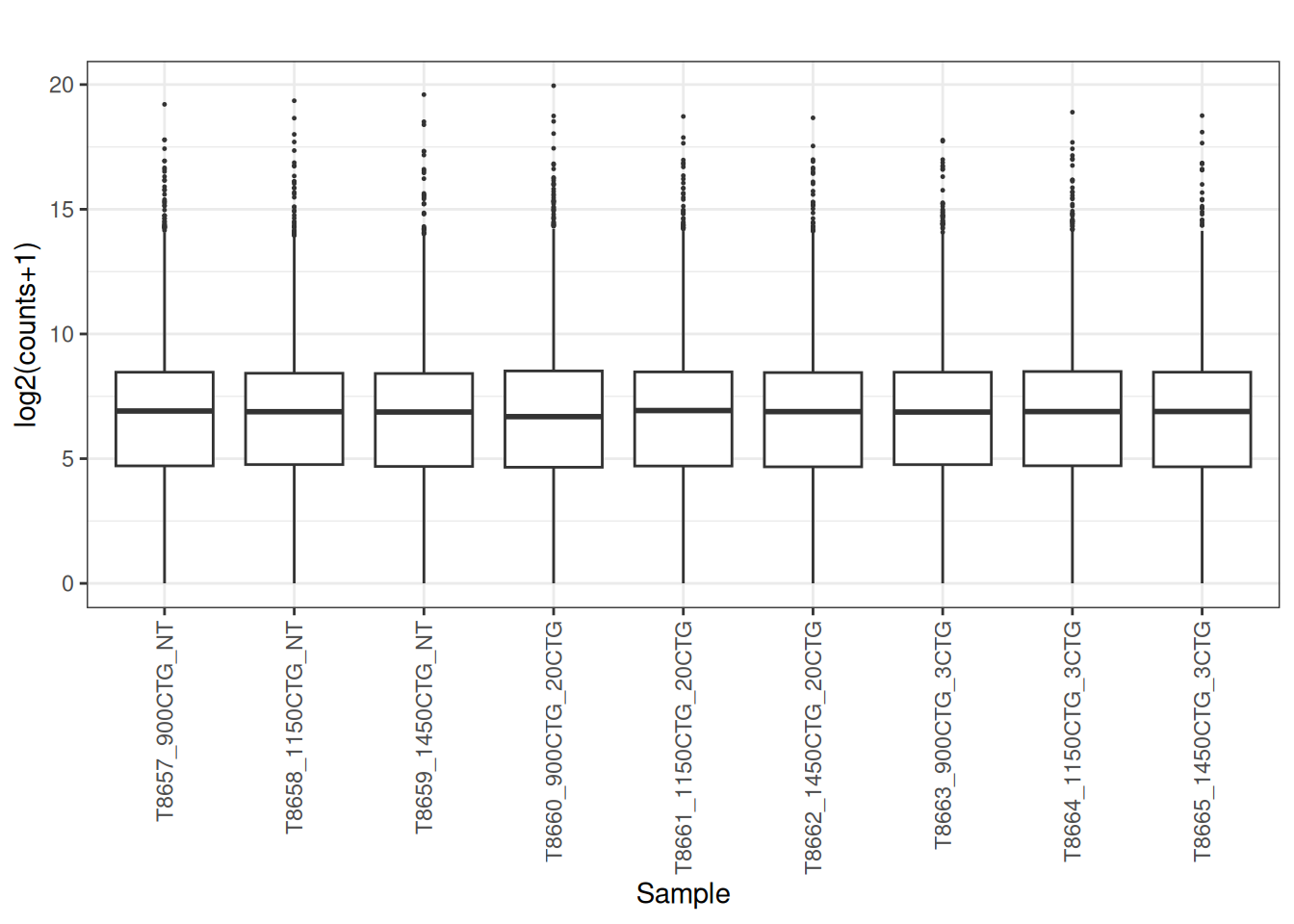
5.5 filter out lowly expressed genes
to_remove <- edgeR::filterByExpr(x_cpm,min.count = 3)
x_cpm_filtered <- x_cpm[to_remove,]
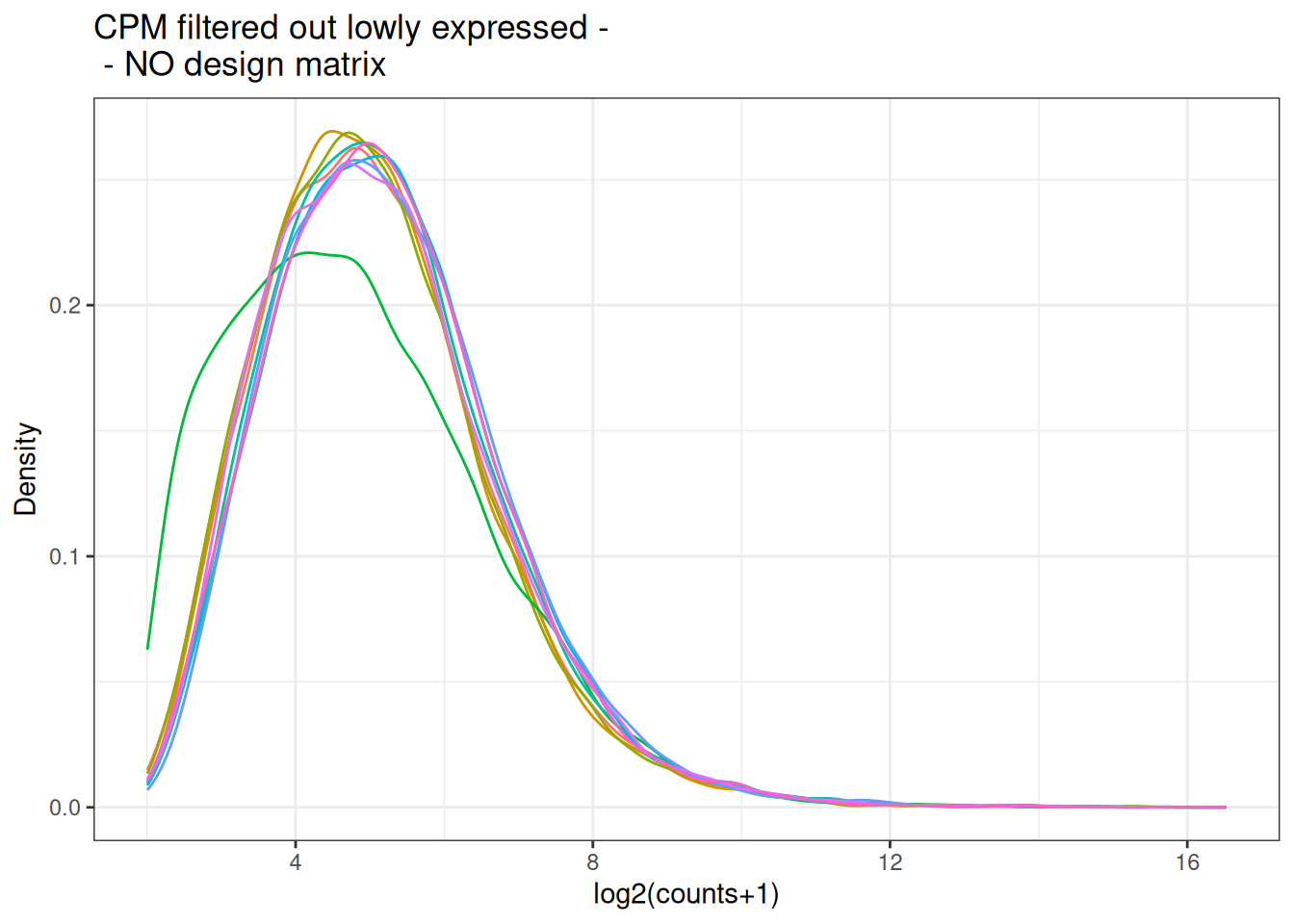
plot_box(x_cpm_filtered,main = "CPM filtered out lowly expressed - \nNO design matrix")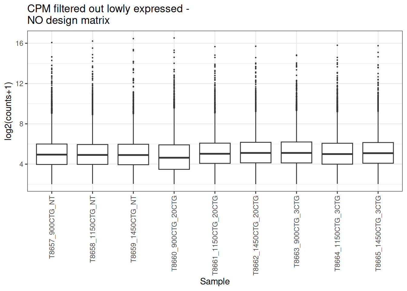
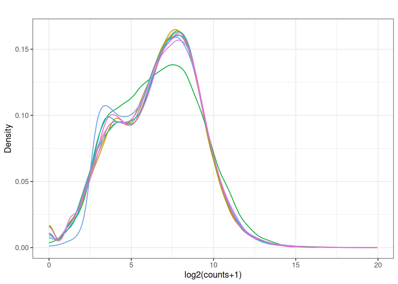
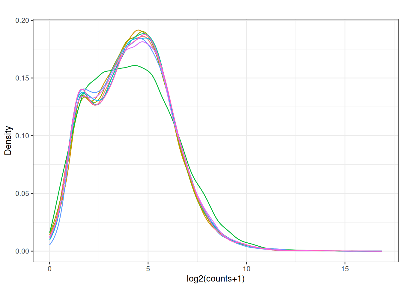
visualize this as density plot as well.
5.6 Incorporate a design matrix - description of the samples.
The above was usingn all of the samples the same but this dataset has varying sample types. I might be hard to figure it out just from column names as they are not so informative but let’s just guess
##  [1] "Gene"                "T8657_900CTG_NT"     "T8658_1150CTG_NT"
##  [4] "T8659_1450CTG_NT"    "T8660_900CTG_20CTG"  "T8661_1150CTG_20CTG"
##  [7] "T8662_1450CTG_20CTG" "T8663_900CTG_3CTG"   "T8664_1150CTG_3CTG"
## [10] "T8665_1450CTG_3CTG"
#design matrix -
samples <- colnames(x)[2:ncol(x)]
patient <- unlist(lapply(samples,FUN = function(x){unlist(strsplit(x,split = "_"))[2]}))
celltype <- unlist(lapply(samples,FUN = function(x){unlist(strsplit(x,split = "_"))[3]}))
sample_data <- data.frame(samples, patient, celltype)
design <- model.matrix(~ 0 + celltype,data = sample_data)
rownames(design) <- sample_data$samples
colnames(design) <- paste0("celltype", levels(factor(celltype)))
design## celltype20CTG celltype3CTG celltypeNT
## T8657_900CTG_NT 0 0 1
## T8658_1150CTG_NT 0 0 1
## T8659_1450CTG_NT 0 0 1
## T8660_900CTG_20CTG 1 0 0
## T8661_1150CTG_20CTG 1 0 0
## T8662_1450CTG_20CTG 1 0 0
## T8663_900CTG_3CTG 0 1 0
## T8664_1150CTG_3CTG 0 1 0
## T8665_1450CTG_3CTG 0 1 0
## attr(,"assign")
## [1] 1 1 1
## attr(,"contrasts")
## attr(,"contrasts")$celltype
## [1] "contr.treatment"Filter use design information
to_remove_withdesign <- edgeR::filterByExpr(x_cpm,
                                            min.count = 3,
                                            design = design)
x_cpm_filtered_withdesign <- x_cpm[to_remove_withdesign,]

colnames(x_cpm_filtered_withdesign ) <- paste(sample_data$celltype,
                                              1:nrow(sample_data),sep = "_")

plot_box(x_cpm_filtered_withdesign,
         main = "CPM filtered out lowly expressed - \n - with design matrix")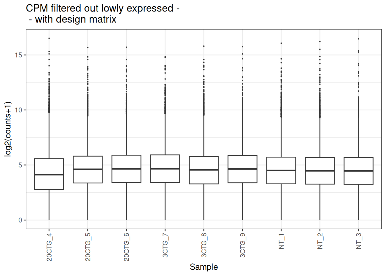
plot_density(x_cpm_filtered_withdesign,main = "CPM filtered out lowly expressed - \n - with design matrix")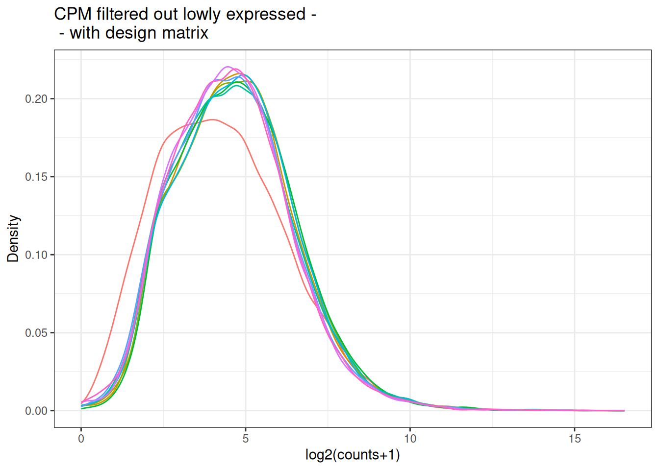
5.7 Normalize Dataset using TMM
library(edgeR)

dge <- DGEList(counts = x[,2:ncol(x)])
dge_filtered <- dge[filterByExpr(dge),]
dge_filtered  <- calcNormFactors(dge_filtered , method = "TMM")
norm_cpm <- cpm(dge_filtered , log = FALSE, prior.count = 1)

plot_box(norm_cpm)
5.8 Look at the distribution of our samples in 2D space
y <- dge_filtered

plotMDS(y, top = 500, labels = colnames(y),
       col = as.integer(y$samples$group))
legend("topright", legend = levels(y$samples$group),
       col = seq_along(levels(y$samples$group)), pch = 16, bty = "n")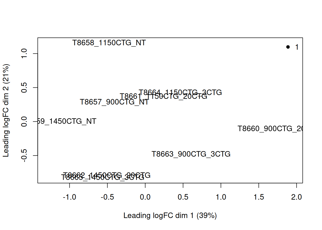
Now incorporate the design into the process
dge <- DGEList(counts = x[,2:ncol(x)],group = sample_data$celltype)
dge_filtered <- dge[filterByExpr(dge),]
dge_filtered  <- calcNormFactors(dge_filtered , method = "TMM")
norm_cpm <- cpm(dge_filtered , log = FALSE, prior.count = 1)

plot_box(norm_cpm)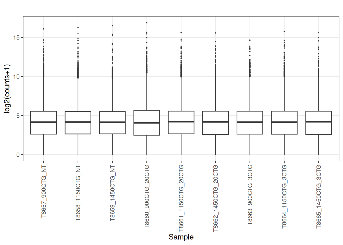

y <- dge_filtered

plotMDS(y, top = 500, labels = sample_data$celltype,#colnames(y),
       col = as.integer(y$samples$group))
legend("topright", legend = levels(y$samples$group),
       col = seq_along(levels(y$samples$group)), pch = 16, bty = "n")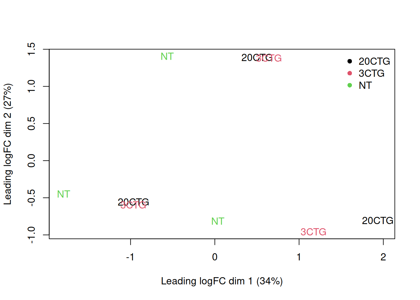
Now incorporate the design into the process
dge <- DGEList(counts = x[,2:ncol(x)],group = sample_data$patient)
dge_filtered <- dge[filterByExpr(dge),]
dge_filtered  <- calcNormFactors(dge_filtered , method = "TMM")
norm_cpm <- cpm(dge_filtered , log = FALSE, prior.count = 1)

plot_box(norm_cpm)
y <- dge_filtered

plotMDS(y, top = 500, labels = sample_data$patient,#  colnames(y),
       col = as.integer(y$samples$group))
legend("topright", legend = levels(y$samples$group),
       col = seq_along(levels(y$samples$group)), pch = 16, bty = "n")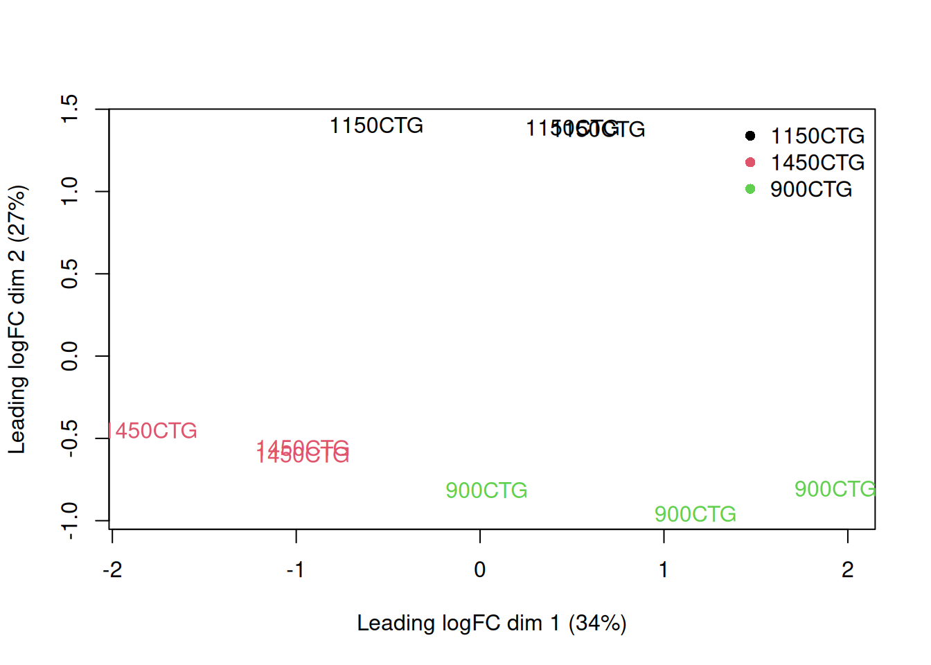
5.9 Normalize the Dataset using RLE
library(DESeq2)

counts <- x[,2:ncol(x)]

keep <- rowSums(counts >= 10) >= 2
counts_filtered <- counts[keep, ]

dds <- DESeqDataSetFromMatrix(countData = counts_filtered,
                              colData = sample_data,
                              design = design)
dds <- estimateSizeFactors(dds)

norm_counts <- counts(dds, normalized = TRUE)

plot_box(norm_counts)