Chapter 5 Worked examples with before/after tables

This chapter shows what the data look like, what the IDs look like, and how the table changes once mapped.

library(knitr)
library(dplyr)

## 
## Attaching package: 'dplyr'

## The following objects are masked from 'package:stats':
## 
##     filter, lag

## The following objects are masked from 'package:base':
## 
##     intersect, setdiff, setequal, union

library(tibble)

kable_head <- function(x, n = 5, caption = NULL) {
  knitr::kable(utils::head(x, n), caption = caption)
}

strip_ensembl_version <- function(x) sub("\\..*$", "", x)

5.1 GSE233947

5.1.1 Raw data preview

source("./fetch_geo_supp.R")
fetch_geo_supp(gse = params$gse)

## Setting options('download.file.method.GEOquery'='auto')

## Setting options('GEOquery.inmemory.gpl'=FALSE)

## Using locally cached version of supplementary file(s) GSE233947 found here:
## data/GSE233947/GSE233947_FeatureCounts_V31genes_RawCounts_ENSG.tsv.gz

## Using locally cached version of supplementary file(s) GSE233947 found here:
## data/GSE233947/GSE233947_modulize_3CTG_20CTG_junctions.tsv.gz

## Using locally cached version of supplementary file(s) GSE233947 found here:
## data/GSE233947/GSE233947_modulize_NT_20CTG_junctions.tsv.gz

## Using locally cached version of supplementary file(s) GSE233947 found here:
## data/GSE233947/GSE233947_modulize_NT_3CTG_junctions.tsv.gz

path <- file.path("data", params$gse)
files <- list.files(path, pattern = params$file_grep, 
                    full.names = TRUE, recursive = TRUE)

kable_head(tibble(file = basename(files)), min(10, length(files)), paste(params$gse,": extracted file list (first 10)"))

(#tab:get_data)GSE233947 : extracted file list (first 10)

file
GSE233947_FeatureCounts_V31genes_RawCounts_ENSG.tsv.gz
GSE233947_modulize_3CTG_20CTG_junctions.tsv.gz
GSE233947_modulize_NT_20CTG_junctions.tsv.gz
GSE233947_modulize_NT_3CTG_junctions.tsv.gz

Raw table preview

library(readr)

safe_read <- function(file) {
  # First attempt: read as TSV
  df <- tryCatch(
    readr::read_tsv(file, show_col_types = FALSE),
    error = function(e) NULL   # catch fatal errors
  )
  
  # If read_tsv failed entirely:
  if (is.null(df)) {
    message("TSV read failed — reading as space-delimited file instead.")
    return(readr::read_table(file, show_col_types = FALSE))
  }
  
  # If read_tsv returned but with parsing issues:
  probs <- problems(df)
  if (nrow(probs) > 0) {
    message("Parsing issues detected in TSV — reading as space-delimited file instead.")
    return(readr::read_table(file, show_col_types = FALSE))
  }
  
  # If everything was fine:
  return(df)
}

x <- safe_read(files[1])


kable_head(x[, 1:min(6, ncol(x))], 5, paste(params$gse,": raw table preview"))

(#tab:preview_raw)GSE233947 : raw table preview

Gene	T8657_900CTG_NT	T8658_1150CTG_NT	T8659_1450CTG_NT	T8660_900CTG_20CTG	T8661_1150CTG_20CTG
ENSG00000108821	456397	486088	608151	2012962	379186
ENSG00000265150	170681	299425	286295	747000	210962
ENSG00000164692	169781	190854	263391	869194	180006
ENSG00000265735	78113	121697	113379	532435	112977
ENSG00000259001	55081	78811	73032	353442	100823

ID preview

id_col <- names(x)[1]
ids <- x[[1]] |> as.character()
kable_head(tibble(raw_id = head(ids, 10), 
                  stripped = strip_ensembl_version(head(ids, 10))), 
           10, paste(params$gse,": ID preview"))

(#tab:id_preview)GSE233947 : ID preview

raw_id	stripped
ENSG00000108821	ENSG00000108821
ENSG00000265150	ENSG00000265150
ENSG00000164692	ENSG00000164692
ENSG00000265735	ENSG00000265735
ENSG00000259001	ENSG00000259001
ENSG00000163359	ENSG00000163359
ENSG00000115414	ENSG00000115414
ENSG00000168542	ENSG00000168542
ENSG00000251562	ENSG00000251562
ENSG00000155657	ENSG00000155657

5.1.2 After mapping (Ensembl → HGNC)

if (any(grepl("^ENSG", strip_ensembl_version(ids)))) {
  library(biomaRt)
  ensembl_ids <- unique(strip_ensembl_version(ids))
  ensembl <- useMart("ensembl", dataset = "hsapiens_gene_ensembl")

  map <- getBM(
    attributes = c("ensembl_gene_id", "hgnc_symbol"),
    filters = "ensembl_gene_id",
    values = ensembl_ids,
    mart = ensembl
  )

  kable_head(map, 10, paste(params$gse,": mapping preview"))

  expr_mapped <- x %>%
    mutate(ensembl_gene_id = strip_ensembl_version(.data[[id_col]])) %>%
    left_join(map, by = "ensembl_gene_id") %>%
  dplyr::select( ensembl_gene_id,hgnc_symbol, everything())


  kable_head(expr_mapped[, 1:min(8, ncol(expr_mapped))], 5, paste(params$gse,": mapped table preview"))
}

(#tab:after_map)GSE233947 : mapped table preview

ensembl_gene_id	hgnc_symbol	Gene	T8657_900CTG_NT	T8658_1150CTG_NT	T8659_1450CTG_NT	T8660_900CTG_20CTG	T8661_1150CTG_20CTG
ENSG00000108821	COL1A1	ENSG00000108821	456397	486088	608151	2012962	379186
ENSG00000265150	NA	ENSG00000265150	170681	299425	286295	747000	210962
ENSG00000164692	COL1A2	ENSG00000164692	169781	190854	263391	869194	180006
ENSG00000265735	RN7SL5P	ENSG00000265735	78113	121697	113379	532435	112977
ENSG00000259001		ENSG00000259001	55081	78811	73032	353442	100823

Summarize the mapping

n_ensembl_total <- expr_mapped %>%
  distinct(ensembl_gene_id) %>%
  nrow()

n_mapped <- expr_mapped %>%
  filter(!is.na(hgnc_symbol), hgnc_symbol != "") %>%
  distinct(ensembl_gene_id) %>%
  nrow()

n_unmapped <- n_ensembl_total - n_mapped

mapping_summary <- tibble::tibble(
  category = c("Total Ensembl IDs", "Mapped to HGNC", "Unmapped"),
  n = c(n_ensembl_total, n_mapped, n_unmapped)
)

mapping_summary

## # A tibble: 3 × 2
##   category              n
##   <chr>             <int>
## 1 Total Ensembl IDs 62248
## 2 Mapped to HGNC    40176
## 3 Unmapped          22072

unmapped_ids <- expr_mapped %>%
  distinct(ensembl_gene_id, hgnc_symbol) %>%
  filter(is.na(hgnc_symbol) | hgnc_symbol == "") %>%
  pull(ensembl_gene_id) %>%
  unique()

length(unmapped_ids)

## [1] 22072

library(stringr)

unmapped_classified <- tibble::tibble(id = unmapped_ids) %>%
  mutate(type = case_when(
    str_detect(id, "^ENSG\\d+$") ~ "Ensembl gene ID (ENSG)",
    str_detect(id, "^ENSG\\d+\\.\\d+$") ~ "Ensembl gene ID with version (ENSG.x) — needs stripping",
    str_detect(id, "^ENST\\d+") ~ "Ensembl transcript ID (ENST) — wrong target for gene mapping",
    str_detect(id, "^ENSP\\d+") ~ "Ensembl protein ID (ENSP) — wrong target",
    str_detect(id, "^ENS.*G\\d+") ~ "Non-human Ensembl gene (e.g., ENSMUSG...) — wrong organism",
    str_detect(id, "^ERCC-") ~ "ERCC spike-in control — not a gene",
    str_detect(id, "^MT-|^mt-") ~ "Mitochondrial gene symbol (not Ensembl ID) — different ID system",
    str_detect(id, "^\\d+$") ~ "Entrez Gene ID — different ID system",
    TRUE ~ "Other / unknown format"
  ))

unmapped_classified %>% count(type) %>% arrange(desc(n))

## # A tibble: 1 × 2
##   type                       n
##   <chr>                  <int>
## 1 Ensembl gene ID (ENSG) 22072

# Use the same mart/dataset as your mapping step:
# ensembl <- useMart("ensembl", dataset = "hsapiens_gene_ensembl")

ensg_details <- getBM(
  attributes = c(
    "ensembl_gene_id",
    "gene_biotype",
    "external_gene_name"
  ),
  filters = "ensembl_gene_id",
  values  = unmapped_ids,
  mart    = ensembl
)

head(ensg_details)

##   ensembl_gene_id                       gene_biotype external_gene_name
## 1 ENSG00000093100                             lncRNA                   
## 2 ENSG00000124593                     protein_coding                   
## 3 ENSG00000124835                             lncRNA                   
## 4 ENSG00000141979                     protein_coding                   
## 5 ENSG00000149656 transcribed_unprocessed_pseudogene                   
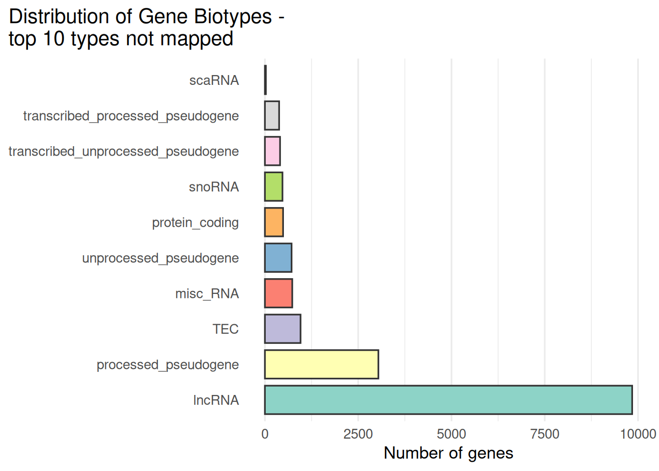
## 6 ENSG00000151303                             lncRNA

Output the distribution of biotypes for the subset of ensembl ids that have no HGNC ID.

library(ggplot2)
x <- ensg_details$gene_biotype
x[is.na(x)] <- "Unknown"

# Base R counts table -> data.frame
tab <- table(x)
df_counts <- data.frame(
  biotype = names(tab),
  n       = as.integer(tab),
  stringsAsFactors = FALSE
)

# Order by counts (ascending) for a nice horizontal bar chart
df_counts <- df_counts[order(df_counts$n,decreasing = TRUE), ]
df_counts$biotype <- factor(df_counts$biotype, levels = df_counts$biotype)

#only include the top 20 biotypes
df_counts <- df_counts[1:min(10, nrow(df_counts)), ]

ggplot(df_counts, aes(x = biotype, y = n, fill = biotype)) +
  geom_col(width = 0.8, color = "grey20") +
  coord_flip() +
  scale_fill_brewer(palette = "Set3", guide = "none") +
  labs(
    x = NULL, y = "Number of genes",
    title = "Distribution of Gene Biotypes - \ntop 10 types not mapped"
  ) +
  theme_minimal(base_size = 13) +
  theme(
    plot.title.position = "plot",
    panel.grid.major.y = element_blank()
  )

Would the mapping of these identifiers have been different if we used a different version of Ensembl?